Time Series Analysis and Stock Price Forecasting Using R

Time series analysis is a specialized statistical technique used to analyze data points collected at consistent intervals over a defined period. Unlike datasets gathered sporadically or arbitrarily, time series data focuses on observations made at regular time steps, allowing analysts to identify patterns, trends, and seasonal variations within the data.

 

Essentially, this method involves examining clearly defined data points generated through continuous and systematic measurement. For instance, a time series might represent monthly retail sales figures or daily temperature readings. In this tutorial, we will explore various time series techniques using the R programming language.

 

Stock price prediction serves as a practical example of time series forecasting. It involves estimating the future value of an individual stock, a specific market sector, or an entire market index. In this study, we will apply several forecasting methods, including the Naive approach, Simple Exponential Smoothing, ARIMA, and Holt’s Trend Model. When the dataset exhibits seasonal fluctuations, advanced models such as Seasonal Naive or TBATS can be employed to improve forecasting accuracy.

 

To demonstrate these techniques, we will use Apple Inc.’s stock price data obtained from Yahoo Finance. The dataset spans approximately 22 years of monthly closing prices, comprising 264 observations across six variables. For this univariate time series analysis, only the closing price variable is utilized, as it provides a reliable indicator for forecasting the subsequent period’s opening price.

Then let's see the packages required to perform the traditional forecasting methods in R:

library(readxl)
library(urca)
library(lmtest)
library(fpp2)
library(forecast)
library(TTR)
library(dplyr)
library(tseries)
library(aTSA)

Read data from an Excel (.xlsx) file into R and inspect the data frame structure for proper data analysis.

AAPL = read_excel("/file_path/AAPL.xlsx")
str(AAPL) # To check the structure of the dataframe 

Before building any predictive model, it’s essential to split the dataset into training and testing sets. Typically, around 80% of the data is allocated for training the model, while the remaining 20% is reserved for testing its performance and accuracy.

In this case, we divided the dataset into training and testing sets using a class-based approach to ensure consistent and structured data handling.

class = c(rep("TRAIN", 211), rep("TEST",53)) # creating the TRAIN and TEST as class varible

str(class)

AAPL = cbind(AAPL, class)    # Binding the "class" column with the existing AAPL data frame
AAPL

# Splitting the data
train_data = subset(AAPL, class == 'TRAIN')

test_data = subset(AAPL, class  == 'TEST')

Next, we need to convert the dataset into a time series object using the ts() function in R, as illustrated below. This step allows R to recognize the data as sequential observations over time, enabling accurate time series analysis and forecasting.

dat_ts = ts(train_data[,5], start = c(2000,1), end = c(2017,07), frequency = 12)
dat_ts 

The initial output of the model displays error metrics calculated only on the training dataset. However, our goal is to evaluate the model’s performance on unseen data — that is, the test set — to understand how well it can predict future values.

To achieve this, we need to extract the predicted values from the trained model and then calculate the error measures using the test data. For this purpose, we will define custom functions to compute common error metrics such as Mean Absolute Error (MAE) and Root Mean Squared Error (RMSE).

mae = function(actual,pred){

  mae = mean(abs(actual - pred))

  return (mae)
}

RMSE = function(actual,pred){

  RMSE = sqrt(mean((actual - pred)^2))

  return (RMSE)
}

Forecasting models:

Navie Model

The Naive Forecasting Method is one of the simplest yet most practical techniques in time series forecasting. It assumes that the next value in a series will be exactly the same as the most recent observation, making it an easy-to-understand baseline for prediction models. Despite its simplicity, the naive method is often surprisingly effective for data that remains relatively stable over time or shows minimal fluctuations. It requires no complex calculations, parameters, or historical trend analysis, making it an ideal starting point for beginners in R programming and forecasting analysis. Analysts frequently use the naive forecast as a benchmark to evaluate the performance of more advanced models like ARIMA Models.

nav = naive(dat_ts, h = 53)
summary(nav)

df_nav = as.data.frame(nav)

mae(test_data$Close, df_nav$`Point Forecast`)
RMSE(test_data$Close, df_nav$`Point Forecast`)

OUTPUT

Simple Exponential Smoothing

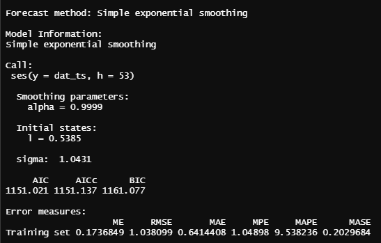
The Simple Exponential Smoothing (SES) method is a popular and effective technique in time series forecasting used to predict future values by giving more weight to recent observations. Unlike the naive approach, which assumes the next value will mirror the last, SES considers the overall trend by smoothing out short-term fluctuations. This makes it especially useful for data without clear trends or seasonal patterns. The method uses a smoothing constant (alpha) to control how quickly the model reacts to changes in the data. In R programming, Simple Exponential Smoothing is widely applied to generate reliable short-term forecasts with minimal complexity.

se_model = ses(dat_ts, h = 53)
summary(se_model)

###

df_s = as.data.frame(se_model)

mae(test_data$Close, df_s$`Point Forecast`)
RMSE(test_data$Close, df_s$`Point Forecast`)

OUTPUT

Holt's Trend Method

The Holt’s Trend Model, also known as Holt’s Linear Trend Method, is an extension of the Simple Exponential Smoothing technique used in time series forecasting. While SES focuses only on the level of the data, Holt’s method adds a trend component, making it more effective for forecasting datasets that show consistent upward or downward movement over time. This model uses two smoothing parameters — one for the level and another for the trend — allowing it to adjust more accurately to long-term changes. In the R code provided below, we demonstrate how to implement Holt’s Trend Model to forecast future values while capturing both stability and direction in the data. This method is ideal for financial forecasting, sales predictions, and other real-world applications where trends play a vital role in decision-making.

holt_model = holt(dat_ts, h = 53)

summary(holt_model)

####
df_h = as.data.frame(holt_model)

mae(test_data$Close, df_h$`Point Forecast`)
RMSE(test_data$Close, df_h$`Point Forecast`)

OUTPUT

ARIMA

The ARIMA (AutoRegressive Integrated Moving Average) model is one of the most powerful and widely used techniques in time series forecasting. Unlike simpler methods such as Naive Forecasting or Simple Exponential Smoothing, ARIMA captures complex patterns by combining autoregression, differencing, and moving averages to make accurate predictions. It is especially effective for datasets that exhibit trends or non-stationary behavior. 

The auto.arima() function in R programming automatically selects the best model parameters by evaluating multiple combinations and choosing the one with the lowest Akaike Information Criterion (AIC) value, ensuring the most efficient fit for the data. In the R code example provided below, we demonstrate how to use the auto.arima() function to build a reliable forecasting model that adapts to the time series’ structure. This method not only enhances forecast precision but also serves as a benchmark for evaluating the performance of other advanced forecasting techniques.

arima_model_AIC = auto.arima(dat_ts,stationary = FALSE, seasonal = FALSE, ic = "aic", stepwise = TRUE, trace = TRUE)

summary(arima_model_AIC)

###
fore_arima = forecast::forecast(arima_model_AIC, h=53)

df_arima = as.data.frame(fore_arima)
df_arima

mae(test_data$Close, df_arima$`Point Forecast`)
RMSE(test_data$Close, df_arima$`Point Forecast`)

OUTPUT

To visualize and compare the results of all the forecasting models, you can use the following code to generate their respective plots.

par(mfrow=c(2,2))
plot(nav)
plot(se_model)
plot(holt_model)
plot(fore_arima)

OUTPUT

Conclusion

The performance of each time series forecasting model was evaluated using two key error metrics — Mean Absolute Error (MAE) and Root Mean Squared Error (RMSE). The results are summarized in the table below:

METHODS	MAE	RMSE
Naive Method	43.46	59.85
Simple Exponential Smoothing	43.46	59.85
Holt’s Trend Method	38.83	54.82
ARIMA	39.33	55.23

Among all the models tested, Holt’s Trend Method achieved the lowest MAE and RMSE values, indicating better accuracy compared to the Naive, Simple Exponential Smoothing, and ARIMA models. This suggests that Holt’s method provides a more reliable forecast for this dataset.

However, it’s important to note that these results are based solely on error measures. While lower errors indicate higher precision, no model can predict future values with absolute certainty — forecasts always carry a degree of uncertainty proportional to the observed error.

To explore the complete R Markdown source code used for this analysis, visit my GitHub repository -